
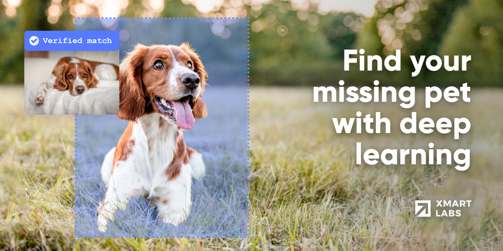
Losing a pet can be a dramatic situation some families might go through. Immediately, social media posts with pictures of the pet emerge from both the owner and the finder. What happens then depends on multiple factors, such as their friends in common, if they share a social group, or even if they use the same social media networks. The connection may or may never happen.
Here at Xmartlabs, we wanted to facilitate the matching by researching deep learning techniques to take the pets back to their homes.
Deep Learning Model
The paper “A Deep Learning Approach for Dog Face Verification and Recognition” [1] proposes a solution to matching two different pictures of the same dog in a large dataset. By training a convolutional neural network, we can transform a 224x224 color image into a feature vector of length 32. Each numeric element of this feature vector represents a characteristic of the dog, so the distance between two vectors represents how similar they are.
The CNN is based on Res-Net [2] as it has residual layers to allow a deeper network and prevent vanishing gradients during backpropagation. According to the authors the net tends to overfit very fast, so they had to apply different strategies to avoid it in training such as dropout layers, data augmentation, and hard triplets (I will explain this one below).
Training and Evaluating the Model
A public dataset and the source code that comes with the paper allowed us to easily train and test our own model. The dataset is composed of multiple pictures of different dogs, where each dog has around four pictures from different angles and backgrounds. Since the paper’s publication, the dataset has grown bigger, and the images went up from 104x104 pixels to 224x224 pixels.
To evaluate the model in a more real-life use case scenario, we divided the dataset into three, one for training, another for evaluation during training, and one for testing the final model. The whole dataset contains 1393 different dogs, which after shuffling were split, leaving 80% for training, 10% for validation, and 10% for testing.
For training, the model uses triplet loss. The idea behind this loss function is to take triplets containing two different images of the same dog, named anchor and positive samples, and another dog picture, named negative sample. Then the model defines the embeddings, trying to get the anchor and positive vectors closer together while getting the negative image further apart.
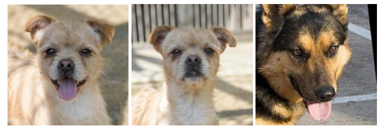
Example of a triplet, from left to right: Anchor sample, positive sample, and negative sample.
The equation for triplet loss is:
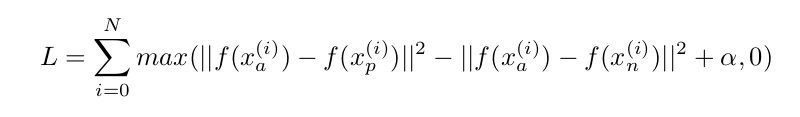
Where xa, xp , and xn represent the anchor, positive and negative samples, respectively, and the function f represents the embedding of the image sample. So that equation says that if the positive sample is closer than the negative (by a distance α) then the embedding is acceptable, if not, there is something to change in the network.
The training loop builds hard triplets to reduce overfitting. These triplets contain the most “difficult” cases by taking the most different anchor, a positive pair, and the negative sample most similar to the anchor. So in a given moment, the network takes some random classes of dogs, gets its embeddings, and checks which triplets might be the most complex cases to resolve in the next step of the training. The number of hard triplets in the batch grows as the accuracy grows.
The network was trained for 250 epochs, on CPU. According to the paper, a longer training would incur overfitting, which was verified in our training. Higher accuracy in validation is attributed to the data augmentation and the generation of hard triplets.
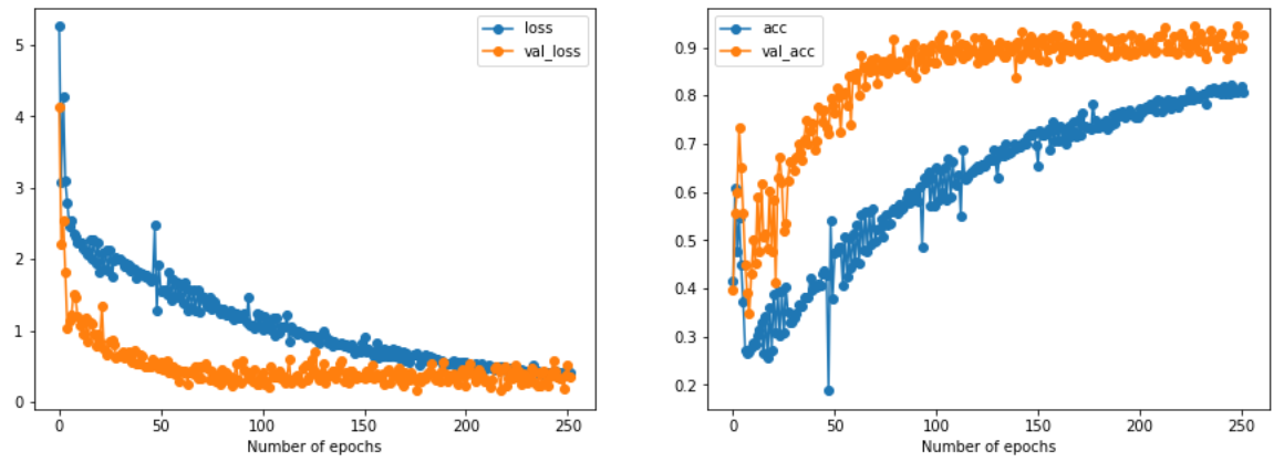
Learning curves, loss and accuracy evolution.
Once the model was fully trained we took 10000 pairs of images, half containing the same dog and half different dogs. Measuring the distance between each pair we calculate the threshold which gives the highest accuracy in deciding if a pair is of the same dog or not. Our results give:
Best threshold: 1.106
Best accuracy: 0.900
While the results presented in the paper are:
Best threshold: 0.063
Best accuracy: 0.920
The confusion matrix and the ROC curve:
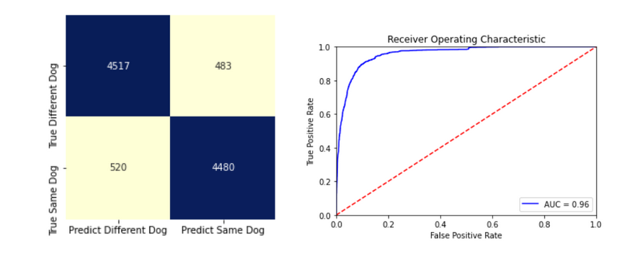
The chosen threshold balances the false negatives and false positives.
It’s interesting to observe where the algorithm is making mistakes and understand what might be the reason.
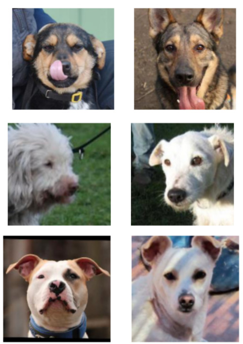
False positive examples.
Although the difference between those dogs might be obvious to a human, we can see a pattern with these mistakes. These examples show that the classifier is taking great importance in the color of the fur, the three cases shown demonstrate that when the faces have a similar color scheme the classifier might get confused.
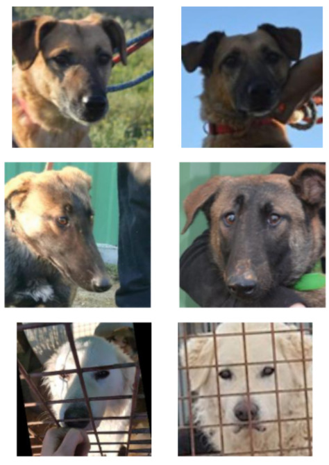
False negative examples.
These false negative examples show that the model isn’t robust enough to detect a match from photos taken with different angles, the same goes for lighting conditions. Some other conditions make recognition even more difficult (such as the dog sticking its tongue or being behind a fence).
As the paper states, once the embedding is done, the idea is to take an image of an unknown dog and label it by its nearest neighbors. To test the performance, all but one image per class in validation were used to train a k-nn model, and by randomly selecting an image the model was tested. This test is performed multiple times because the images sampled can change the results.
Labeling by the nearest neighbor, the accuracy is around 0.48, which results in a much lower accuracy than the problem of determining if a pair is the same dog or not. This is because the first problem is less complex as it has a 50% chance of being correctly labeled, while the classification problem has 139 possible classes.
To make the classification easier, the paper shows the rank-k classification. This is done by doing the same split in the validation dataset, then instead of keeping the label of the nearest neighbor, we take the k closest labels, this means that if for example, the two nearest neighbors correspond to the same dog, then this counts as one.
![]()
This increases the accuracy substantially, and it might be a more accurate representation of the case of use of this model, as it would be reasonable for the user to upload an image, and then the program gives more than one possible match, leaving the user to make the final decision.
These tests were done representing a case where the database would have many images of a dog and later one image would be fitted to those appearing in the dataset. In reality, we would have many images of a dog in the database and many images of the same dog to fit, this would give a more robust system, as taking the nearest classes for each input image gives more possibilities and if one image has an issue (the photo was taken from a strange angle, the dog is behind a fence, etc.) the other images would be helpful.
Conclusions
After reviewing this paper and putting it to the test, we conclude that the results look promising. It shows some scaling issues, but with the correct implementation inside a program, it can help find a dog inside a large dataset of images. It is also important to note that the model is adaptable to other clustering problems, and it's not only suitable for dogs. We recommend reading "Pet Cat Face Verification and Identification" [3] and "FaceNet: A Unified Embedding for Face Recognition and Clustering" [4]. These papers study the same problem but for cats' and humans' faces, respectively.
This is just a computer vision approach to automate dog identification. If you have something to automate, predict, or optimize, we can explore machine learning solutions together to turn it into reality. Like what you read? Stay tuned to upcoming content related to machine learning and computer vision solutions for real-life issues.
Bibliography
- Mougeot, Guillaume & Li, Dewei & Jia, Shuai. (2019). A Deep Learning Approach for Dog Face Verification and Recognition. 10.1007/978-3-030-29894-4_34.
- He, K., Zhang, X., Ren, S., Sun, J.: Deep residual learning for image recognition. CoRR abs/1512.03385 (2015). http://arxiv.org/abs/1512.03385
- Klein, Adam. Pet Cat Face Verification and Identification. 2015. http://cs230.stanford.edu/projects_fall_2019/reports/26251543.pdf
- Schroff, F., Kalenichenko, D., Philbin, J.: FaceNet: a unified embedding for face recognition and clustering. CoRR abs/1503.03832 (2015). http://arxiv.org/abs/1503.03832

