
Kaggle competitions attract thousands of data science and machine learning enthusiasts by providing access to various datasets and infrastructure with GPU availability and discussion forums to share ideas; this is very important for practitioners looking for a starting point.
Here at XmartLabs, we're always looking for ways to contribute to real problems that have a genuine impact on people. Kaggle is an excellent example of this because it gives organizations a platform to present their issues so that savvy technical people can solve them.
For this competition, the NFL wanted to find a solution to a critical problem they have: Player's Health & Safety. This is not the first time they have cooperated with Kaggle; they set out to identify helmet impacts in a previous competition. This time around, they wanted to determine which helmet belongs to each player and keep track of their collisions through a match. Currently, the tracking is done by hand, but an automated algorithm would significantly reduce the time needed to do it manually, freeing more resources to do complex research about how to ensure players' safety in the field. In this blog post, the NFL gives its statement on the importance of this competition.
The Challenge
The dataset has two sources of information, the videos, and the tracking information. The objective is to match the detected helmets in each video frame to the label of its corresponding player, which are identified by their shirt number and whether they're in the home or visitor team; some examples of players' labels are 'H67' or 'V9'.
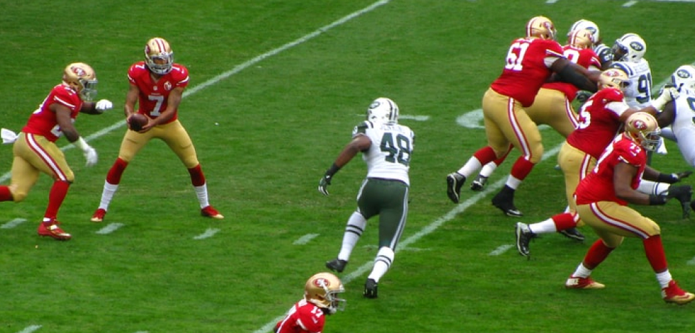
The video training datasets consist of 60 short plays (around 10 seconds videos with 60 fps). Each play is filmed from two synchronized cameras, one located at the endzone and the other one at the sideline, concluding in a total of 120 videos in the training dataset.
Left image: SidelinView. Right image: Endzone view.
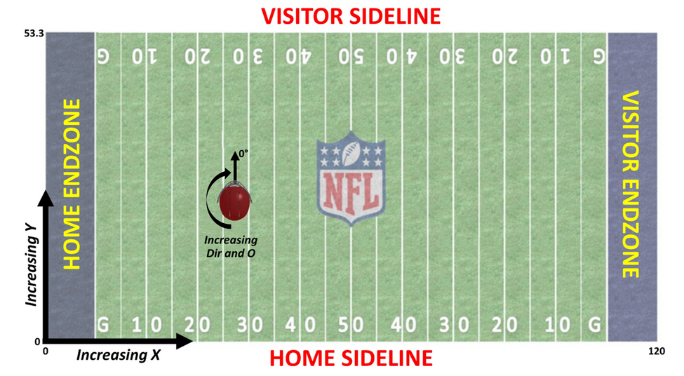
The tracking information comes from a device located in the player's shoulder pad. It gives the relative position of each player on the field with other information about the player's movement at a 10Hz frequency. The tracking has the 'x' and 'y' positions described in the image below.
Other supplementary information given in tracking is speed, acceleration, distance traveled from the last point, and orientation. Below, you can see an example of the player's position at the beginning of a game.
Another file given at the start of the competition was the location of the helmets in a given frame, predicted by a baseline model. These predictions are not perfect; the reason for giving them is to provide competitors with a starting point independently from the detection of helmets to focus on the real problem. The training images are given so you can train your own helmet detector, and although we didn't take this approach, some top-scoring teams did. There's an interesting discussion around this topic because top-scoring competitors tried the same solution but with the baseline helmet detector and found a 10% decrease in the score.
Our Solution
Our solution is made of many sequential modules, and each of them tackles a specific task. These modules can be worked on individually, allowing us to develop and fix some of them in parallel. We order the modules by importance and complexity:
1. 2D Matching:
The central part of this problem is mapping the helmet's positions in a given frame with the tracking coordinates. As both sources of information are in a two-dimensional space, the mapping has to be done accordingly; what we call '2D Matching'. As simple as it can be for a human to match two clouds of points (with reasonable similarity), there's more than one way to do it automatically on a computer. Various algorithms tried to solve this optimization problem, where the value to optimize is the distance between the matched pairs.
In our case, we used the method proposed in the paper "Robust Point Set Registration Using Gaussian Mixture Models," which has its code available in Python. With some minor changes, we were able to include it in our solution.
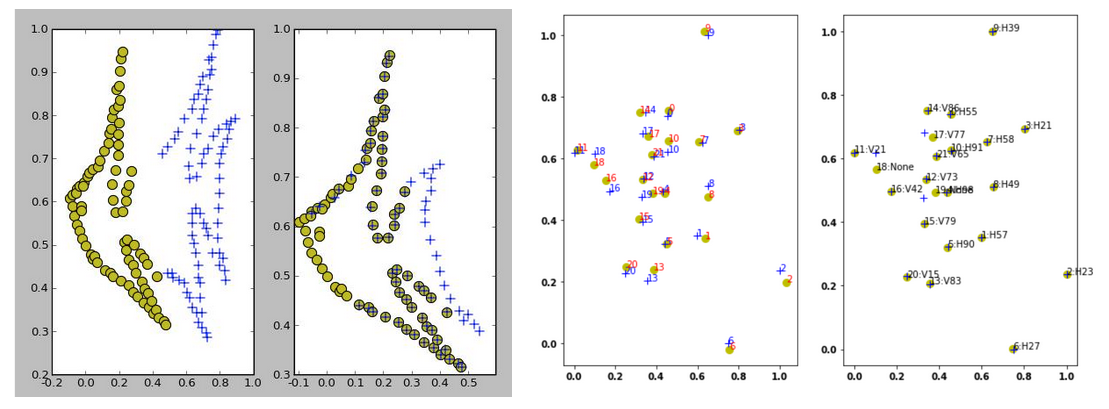
Left: Example shown in code presentation, Right: Example of implementation in our solution.
When passed two normalized clouds of points, the algorithm can return a correspondence between those cloud points. There are some issues; for example, when both sets have 22 points, the algorithm works really well, but when the video has a frame with fewer helmets, the results might have some errors. Because of this, we decided only to do 2D matching when there are 15 helmets or more in the image frame. Later we'll explain how we propagate the labels to the frames that don't have enough helmets. Besides this, we didn't run the matching on all frames, as variations in consecutive frames were almost none.
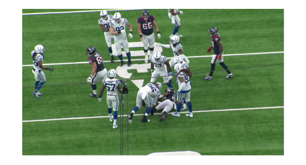
Example of a low number of helmets in the frame.
2. DeepSORT:
Once the matching gets done, we transfer these intermediate results to the DeepSORT module. By using DeepSORT, we add a temporal dependency between the frames of a video. This algorithm is commonly used on object tracking problems; it tries to keep up with a helmet throughout the video by assigning it an ID. Finally, based on the 2D matching results, it looks for the most given label for that helmet and designates it as its final label.
We used an idea to match only in frames we were confident the results would be good. By doing this, DeepSORT took only those certain frames' labels and spread them throughout the video.
3. DeepSORT Correction:
Our output from deepSORT did have errors, so we wanted to come up with a creative solution. One of the main issues were duplicated labels and 'None' labels (when no valid labels were assigned to that helmet). These errors didn't appear on all frames, so we used the frames that had all the helmets matched to correct the other ones. We decided to do a two-step solution, first fixing simple duplicated errors and more significant problems after.
The first step addressed cases where there were only two identifiable errors, a duplicated pair. Assuming that all the other labels were correct, we decided to pick the four closest helmets to one of the duplicates. Using a homography matrix, we transferred the duplicate to the tracking space and found the closest player there. By analyzing the results of each helmet in the pair, we built an algorithm to decide how to correct it.
After fixing those simple errors, we matched each remaining frame with detectable errors and the nearest one without errors. In this case, we used the Hungarian Algorithm to perform the matching.
In some cases, this implementation gave impressive results. As seen in the following video, green bounding boxes are correctly labeled helmets and yellow when there is an impact (higher reward for the correct label while collision). The red bounding boxes are due to wrong labels during a collision.
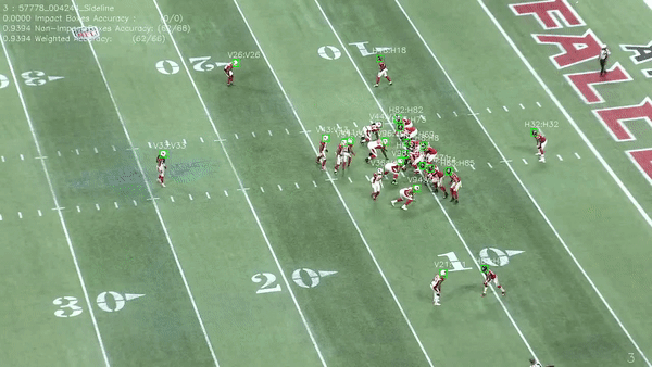
Output of our solution applied to a Sideline video.
4. Image Rotation:
The initial matching was done by doing many iterations looking for the best rotation angle that could fit the helmets in the x-axis with the tracking data. This is very expensive computationally, so we decided to help out the algorithm by finding the best rotation without iterating. After changing the matching, this module was kept since it also helped the '2D-matching'.
Our solution detects the field lines using the Canny edge detector algorithm followed by the Hough line transform. With those detected lines, the rotation angle is calculated. By rotating, we can position the helmets in a way that's more representative of reality.
As seen in the example of the two marked players, the bottom one appears to be more to the right; however, in reality, the top one is further to the right. By doing the rotation, the problem is solved.
The rotation is done using the purple line, and the angle with the green one is the rotation angle.
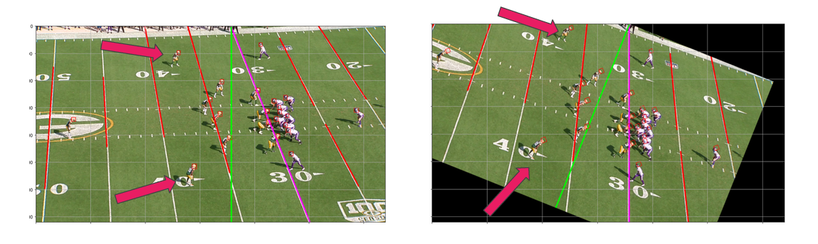
Image rotation example.
5. Outfield players:
Another issue we saw and addressed was the presence of off-field players/helmets. The baseline helmet detector didn't discriminate between these two types of helmets, so some labels were assigned to outfield players. This meant those labels weren't being assigned to the correct player, which generated an offset that moved all labels to another helmet.
To solve this, we detected sideline lines to differentiate these two types of helmets. One difference with image rotation is that, in this case, we looked for wider lines, like the one shown in the image.
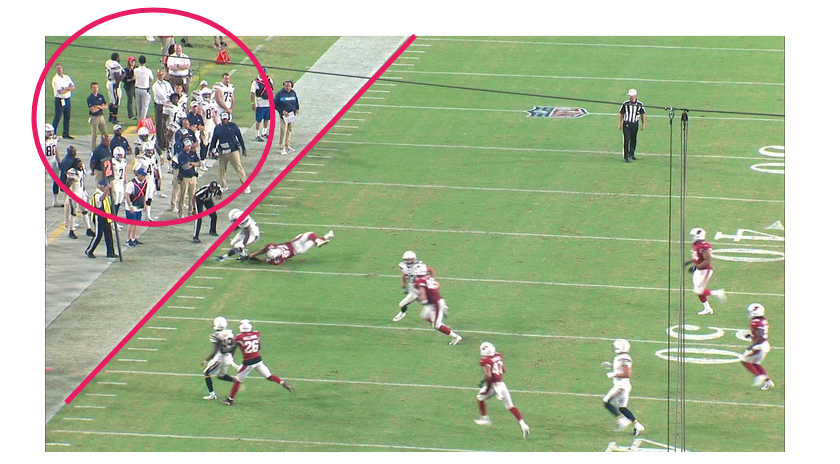
Most of the detected helmets are field players, so considering all helmets as players gives a precision of 0.983. With our detector, precision was improved to 0.994.
6. Camera angle detection:
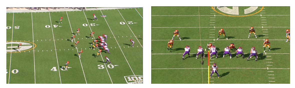
Each video was labeled "Sideline" or "Endzone," but it wasn't specified from which side or field end it was being recorded. There were two possibilities for each. Identifying this quickly and confidently can signify a correction before the matching, which facilitates it and means it needs fewer iterations.
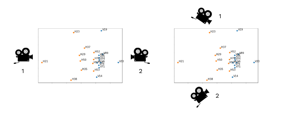
Left: Endzone example. Right: Sideline example.
At the beginning of each video, we saw that the formations were very identifiable and easy to correlate with the tracking. In other words, with the correct view, the 2D matching should have a high rate of matches. So the implementation takes five frames distributed in the first 100 frames. In these selected frames, the 2D matching is done for each possible case; the one with the most matches is selected as correct; after doing it for all five frames, the correct side is selected and saved.
Ideas that didn't make it into the final solution
For different reasons, not everything we tried made it into the final solution. Here we present two of the ideas that didn't.
Team clustering is the idea of separating the helmets by each team. The idea was that the 2D matching algorithm worked better if it had to match 11 helmets with 11 labels twice instead of 22 with 22 once. Our first idea was to use the helmet's color as the colors are very different most of the time. We run tests trying three color spaces: RGB, HSV, and CIELAB.
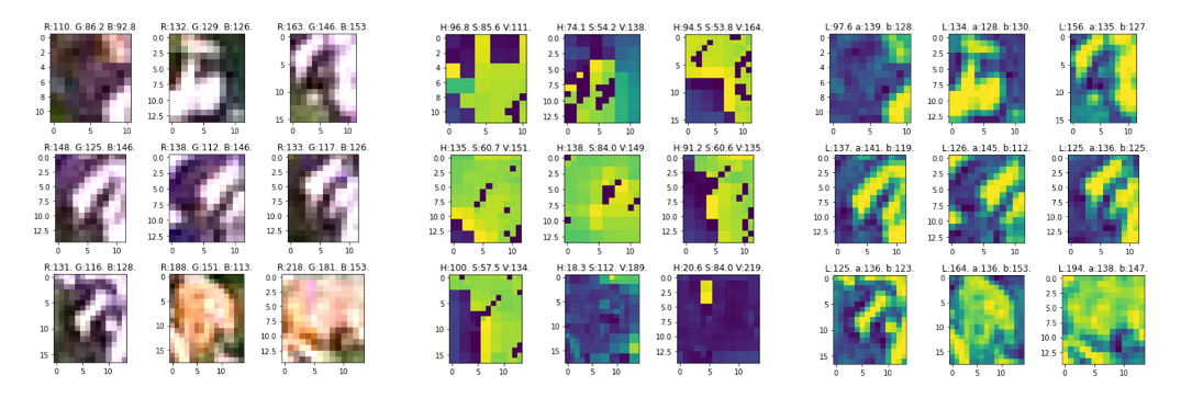
The use of HSV and CIELAB is to get values independent from illumination and other environmental phenomena. Some top scoring solutions did focus on team clustering but with different approaches, for example, using deep learning models.
Although cameras were fixed in a position, they still could rotate and zoom in or out during a play. We tried to capture this information to leverage it in the solution because if we know how the image is moving, we can predict which players are leaving the frame and discard their tracking information. Next, we look at the difference between the first frame of a video and the last.
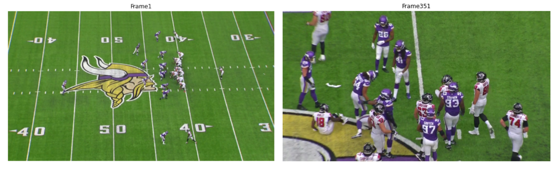
Calculating the size and number of the helmets in the frame, we can have a good approximation of how the zoom is going:
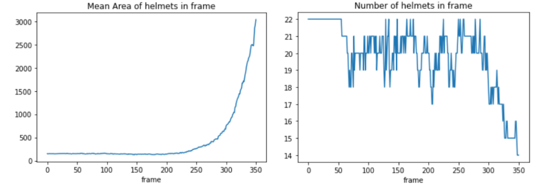
However, merging this information with our pipeline wasn't easy, as more processing had to be done, and at the time, it didn't seem relevant.
Solutions from other competitors
As the competition came to a close, scores on the leaderboard started to soar. Top teams got our attention, and we were looking forward to the end of the competition to see what they had done. Showing your solution and code is optional, but it is common for top Kaggle contestants to share their work.
Looking at other teams, we can confidently say that our ideas weren't that far from top-scoring solutions. In our opinion, the most creative solution was the one that came on top (notebook and explanation are public). On this code, as in many others, a helmet detector was trained. Most of these detectors are YoloV5 architectures trained on the competition's data. However, this one uses a 2-stage detector, whereas the first model resizes the images, and the second one is trained to predict this resized image.
From here on, the code gets more complex, but to keep it simple, we can synthesize the rest of the code as follows:
- Image to Map converter: A Convolutional Neural Network (based on the U-Net) thats' trained to transform the detected helmet's positions into the tracking space.
- Team Classification: With another CNN, the helmets in a frame are processed, and after that, separated into two teams. This classification doesn't predict if the teams are Home or Visitors.
- Points to Points Registration: Using Iterative Closest Points, the best transformation is selected to minimize the distances between both cloud points.
- Tracker: Using IoU tracker, it accumulates the results of player assignment through all frames and re-assigns players to bounding boxes.
- Ensemble: Applying ensemble learning with four models, the final prediction benefits from multiple "opinions."
Other solutions are more ground-based and share points with ours. Looking at them made us realize where we had to emphasize and where we had put too much work.
Conclusion
We want to thank the Kaggle hosts and the NFL for this fantastic competition. Although our solution was among the top 50, we would have loved to prove ourselves further. However, we still had fun trying new stuff and learning a lot along the way. Kaggle is a great place to work on your ML skills, and the community is always open to giving a helping hand. We know that we will do much better the next time by applying what we learned from this experience about competing in a Kaggle competition (you can read about it here).

